MEGA Model Optimization Package
Hal Daume III ( )
)
Fifth Release 17 August 2007
Fourth (b) Release 30 April 2007 -- go here
Fourth Release 10 November 2006
Bug Fix Release 6 April 2006 -- go here
Third Release 17 January 2006 -- go here
Bug Fix Release 30 November 2005 -- go here
Bug Fix Release 23 March 2005 -- go here
Second Release 24 January 2005 -- go here
First Release 20 August 2004 -- go here
Introduction
Maximum entropy models are very popular, especially in natural
language processing. The software here is an implementation of
maximum likelihood and maximum a posterior optimization of the
parameters of these models. The algorithms used are much more
efficient than the iterative scaling techniques used in almost every
other maxent package out there. A description of the algorithms is
available in the following unpublished report:
|
Notes on CG and LM-BFGS Optimization of Logistic Regression
These are notes on this implementaiton of conjugate gradient and
limited memory BFGS optimization for logistic regression (aka maximum
entropy) classifiers. The notes were created because it is actually
quite difficult to find good references on efficient implementation of
these algorithms, though discussion of them exists everywhere.
|
What's New!
New features: You can do passive aggressive updates (ala
Crammer et al.) with perceptron or multitron by specifying -pa. You
can also do instance normalization with -norm1 or -norm2 (for l1 and
l2 norms respectively). You can use named classes (-nc) and finally
everything is about 3-4 times faster!
Bug fix: -nobias works better now (i.e., works at all).
New feature: You can now train using perceptron updates for binary or
"multitron" updates for multiclass problems. For these, the -lambda parameter
is ignored (though it may not be in the future). Performance tends to be
comparable to the binary/multiclass optimization.
New feature: Now, the model spits out the weights that occurred at the
highest dev performance; to restore the old way of spitting out the final
weights, use -lastweight.
New feature: You can do multilabel classification. Specify -multilabel
on the command line and replace class ids with cost vectors. Eg., "0:0:1:2" is
a four class problem for which predicting class 0 and 1 lead to a cost of zero,
predicting class 2 leads to a cost of one and predicting class 3 leads to a
cost of two. Only works with multiclass or multitron optimization.
Speed-up: Approximate Bayes factor feature selection is a lot faster
now.
New feature: Prediction can be run in a dual-pipe mode. If you use "-"
as the name of the file to predict, you can write examples to stdin and read
predictions from stdout. Flushing is forced early, so you can do prediction
one-by-one.
New feature: Compute learning curves (-curve option) without rerunning
megam lots of times.
New feature: You can now do ranking. In particular, if you use
the explicit file format together with -nobias, you can
accomplish a ranking model. Importantly, the number of "classes" does
not need to be the same for each example.
Bug fix: Various errors with the explicit file format.
New feature: All files read either as weights from
-predict or data files can now be compressed. If the file
ends in .Z, .gz or .bz2, it will
automatically read it as a compressed file.
New feature: -nobias option turns off the learning of
a bias parameter.
New feature: the cap on the maximum number of training examples
has increased.
Bug fix: the saving of weights with feature selection was
broken; it now works properly. Thanks to Taichi Nakamura for pointing
this out!
Bug fix: there was a bug with predicting explicit multiclass
data; it should be fixed now. Thanks to Ashish Venugopal for pointing
this out!
Bug fix: using explicit class feature information for multiclass
problems was broken; it is fixed in the new version. Thanks to Simon
Clematide for pointing this out!
Bug fix: there was a small, but important bug with estimating the
bias (stupid bias...it gets me every time). You'll want to get the
new version ASAP. Many thanks to Shou-de Lin for pointing this
out!
There are several changes from version 1 to version 2. First, some
limits (number of examples) has been raised to over four million (and
it's still more than sufficiently efficient with this much data).
Additionally, features have been added for "density
estimation" style modeling (specifically for whole-sentence
maximum entropy language models), restarted training, naive domain
adaptation and feature selection. See options
-prog/-sfile, -mean, -init and
-abffs below.
Code and Executables
The software can be downloaded as source code (in O'Caml) or as executables for i686
Linux or Sun4 Solaris. For executables, there are both debugging
versions and optimized versions avaiable:
Source: megam_src.tgz
Linux: Debugging: megam_i686.gz or Optimized: megam_i686.opt.gz
Solaris: I no longer have access to a sun machine...sorry, download the source.
Windows: I no longer have access to a Windows machine...sorry, download the source.
For people at Utah: The optimized executable can be run as
/home/hal/bin/megam.
This code is free to anyone and you can use it in any research thing
you want. For commercial use, please contact me. If you use it for
work in a published article, please add a footnote acknowledging the
software, or cite the article above.
Speed
I have produced some graphs comparing the efficiency of MegaM to
YASMET, a maxent software package by Franz Josef Och (now at Google),
that uses generalized iterative scaling for optimization. This has
been done both for a binary problem and a multiclass problem, each
with about 140 thousand training instances and 30 thousand test
instances, with hundreds of thousands of features (an NP chunking
task, if you must know).
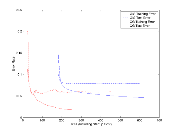
Below, we see training error and test error curves plotted against
time (not number of iterations) for GIS and for CG (our binary
optimizer). Both are done with lambda=1 smoothing. As you can see,
CG both achieves lower error rates, and achieves them more quickly (it
is done after less than 100 seconds, less than the time it takes
YASMET to even start up):

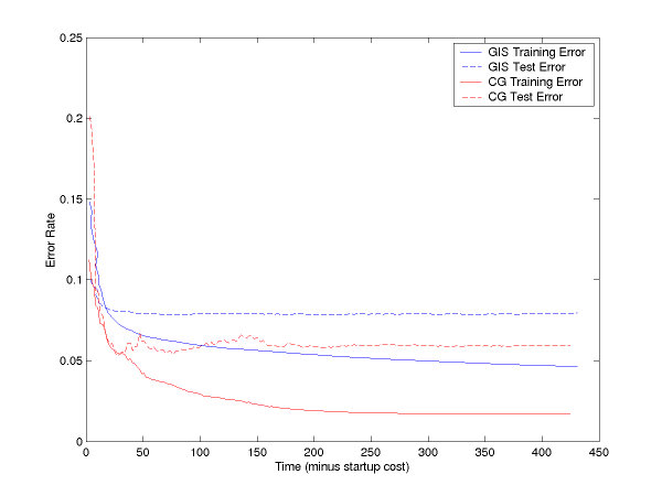
If you subtract off the startup file reading time, the curves are:

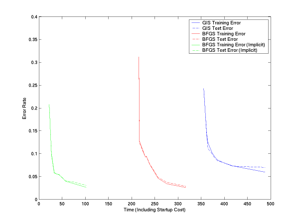
We have done the same thing for multiclass. In this, we have two
versions of LM-BFGS, one which uses explicit feature vectors and one
which uses implicit feature vectors (see usage and file formats
below). Both are faster than GIS, and implicit is quite significantly
faster:

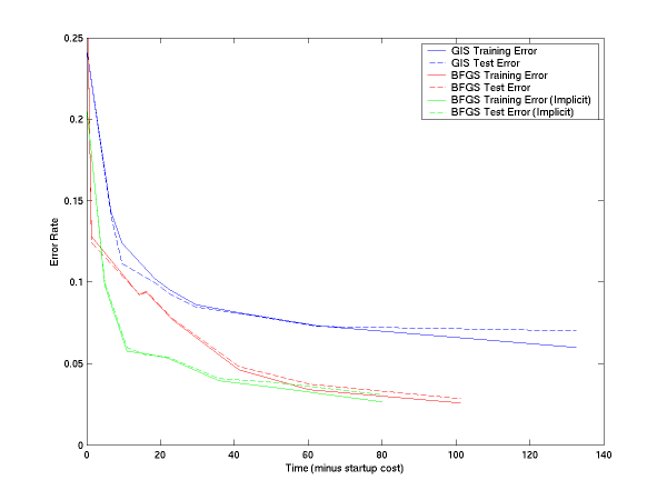
If you subtract off the startup file reading time, the curves are:

Usage
The MegaM software lists its usage if you run it with no (or with
invalid) arguments. Three types of problems can be solved using the
software: binary classification (clases are 0 or 1), binomial
regression ("classes" are real values between 0 and 1; the
model will try to match its predictions to those values), or
multiclass classification (classes are 0, 1, 2, and so on).
usage: megam [options] <model-type> <input-file>
[options] are any of:
   -fvals           data is in not in bernoulli format (i.e. feature
                    values appear next to their features int the file)

   -explicit        this specifies that each class gets its own feature
                    vector explicitely, rather than using the same one
                    independently of class
                    (only valid for multiclass problems)

   -quiet           don't generate per-iteration output

   -maxi <int>      specify the maximum number of iterations
                    (default: 100)

   -dpp <float>     specify the minimum change in perplexity
                    (default: -99999)

   -memory <int>    specify the memory size for LM-BFGS (multiclass only)
                    (default: 5)

   -lambda <float>  specify the precision of the Gaussian prior
                    (default: 1)

   -tune            tune lambda using repeated optimizations (starts with
                    specified -lambda value and drops by half each time
                    until optimal dev error rate is achieved)

   -sprog <prog>    for density estimation problems, specify the program
                    that will generate samples for us (see also -sfile)

   -sfile <files>   for de problems, instead of -sprog, just read from a
                    (set of) file(s); specify as file1:file2:...:fileN

   -sargs <string>  set the arguments for -sprog; default ""

   -sspec <i,i,i>   set the <burn-in time, number of samples, sample space>
                    parameters; default: 1000,500,50

   -sforcef <file>  include features listed in <file> in feature vectors
                    (even if they don't exist in the training data)

   -predict <file>  load parameters from <file> and do prediction
                    (will not optimize a model)

   -mean <file>     the Gaussian prior typically assumes mu=0 for all features;
                    you can instead list means in <file> in the same format
                    as is output by this program (baseline adaptation)

   -init <file>     initialized weights as in <file>

   -abffs <int>     use approximate Bayes factor feature selection; add features
                    in batches of (at most) <int> size

   -curve <spec>    produce a learning curve, where spec = "min,step"
                    and we start with min examples and increase (multiply!)
                    by step each time; eg: -curve 2,2

   -nobias          do not use the bias features

   -repeat <int>    repeat optimization <int> times (sometimes useful because
                    bfgs thinks it converges before it actually does)

   -lastweight      if there is DEV data, we will by default output the best
                    weight vector; use -lastweight to get the last one

   -multilabel      for multiclass problems, optimize a weighted multiclass
                    problem; labels should be of the form "c1:c2:c3:...:cN"
                    where there are N classes and ci is the cost for
                    predicting class i

<model-type> is one of:
   binary           this is a binary classification problem; classes
                    are determined at a threshold of 0.5 (anything
                    less is negative class, anything greater is positive)

   perceptron       binary classification with averaged perceptron

   multitron        multiclass classification with averaged perceptron

   binomial         this is a binomial problem; all values should be
                    in the range [0,1]

   multiclass       this is a multiclass problem; classes should be
                    numbered [0, 1, 2, ...]; anything < 0 is mapped
                    to class 0

   density          this is a density estimation problem and thus the
                    partition function must be calculated through samples
                    (must use -sprog or -sfile arguments, above)
A standard call for optimization would be something like
"megam binary file" or "megam multiclass
file where file is an existing file that contains the
training data (see file formats, below). This will run for at most
100 iterations (for BFGS, when the weight vector doesn't change,
iterations will cease no matter what you specify).
The program will write the learned weights to stdout and will write
progress reports to stderr. For instance, using the small2.gz data set (unzip it first), we get (with
stdout is directed to another file or to /dev/null):
% ./megam.opt multiclass small2 > weights
Scanning file...1000 train, 600 dev, 700 test, reading...done
it 1   dw 3.162e-01 pp 1.09651e+00 er 0.44500 dpp 1.08996e+00 der 0.45000 tpp 1.10488e+00 ter 0.44714
it 2   dw 2.409e-01 pp 7.36678e-01 er 0.17100 dpp 7.05990e-01 der 0.15667 tpp 7.48023e-01 ter 0.17571
it 3   dw 2.620e-01 pp 4.58951e-01 er 0.08500 dpp 4.33894e-01 der 0.06667 tpp 4.65503e-01 ter 0.08857
it 4   dw 2.439e-01 pp 3.20783e-01 er 0.05800 dpp 3.05617e-01 der 0.05500 tpp 3.24992e-01 ter 0.05429
it 5   dw 3.763e-01 pp 2.19297e-01 er 0.03100 dpp 2.05452e-01 der 0.03167 tpp 2.21807e-01 ter 0.02429
it 6   dw 4.723e-01 pp 1.70574e-01 er 0.01300 dpp 1.64530e-01 der 0.01500 tpp 1.72357e-01 ter 0.00857
it 7   dw 2.124e-01 pp 1.46320e-01 er 0.01700 dpp 1.36616e-01 der 0.01500 tpp 1.52102e-01 ter 0.01714
it 8   dw 2.558e-01 pp 1.18902e-01 er 0.01000 dpp 1.12224e-01 der 0.01167 tpp 1.22858e-01 ter 0.00571
it 9   dw 3.500e-01 pp 1.03973e-01 er 0.00800 dpp 9.84038e-02 der 0.01000 tpp 1.07186e-01 ter 0.00429
it 10  dw 1.806e-01 pp 8.78036e-02 er 0.00500 dpp 8.35916e-02 der 0.00667 tpp 9.10291e-02 ter 0.00286
it 11  dw 9.880e-02 pp 7.99700e-02 er 0.00300 dpp 7.63937e-02 der 0.00333 tpp 8.27229e-02 ter 0.00286
it 12  dw 5.143e-01 pp 6.30349e-02 er 0.00100 dpp 6.01651e-02 der 0.00167 tpp 6.45565e-02 ter 0.00143
it 13  dw 1.995e-01 pp 6.02724e-02 er 0.00100 dpp 5.76503e-02 der 0.00167 tpp 6.10948e-02 ter 0.00143
it 14  dw 3.905e-01 pp 5.64137e-02 er 0.00000 dpp 5.32447e-02 der 0.00000 tpp 5.69302e-02 ter 0.00000
it 15  dw 4.482e-02 pp 5.64692e-02 er 0.00000 dpp 5.32684e-02 der 0.00000 tpp 5.69913e-02 ter 0.00000
it 16  dw 4.023e-02 pp 5.63336e-02 er 0.00000 dpp 5.31459e-02 der 0.00000 tpp 5.68540e-02 ter 0.00000
it 17  dw 2.566e-01 pp 5.56057e-02 er 0.00000 dpp 5.24170e-02 der 0.00000 tpp 5.60241e-02 ter 0.00000
it 18  dw 2.695e-01 pp 5.57867e-02 er 0.00000 dpp 5.26410e-02 der 0.00000 tpp 5.61494e-02 ter 0.00000
it 19  dw 9.443e-02 pp 5.53901e-02 er 0.00000 dpp 5.23822e-02 der 0.00000 tpp 5.56894e-02 ter 0.00000
it 20  dw 1.356e-01 pp 5.52823e-02 er 0.00000 dpp 5.22328e-02 der 0.00000 tpp 5.56007e-02 ter 0.00000
it 21  dw 2.865e-01 pp 5.42961e-02 er 0.00000 dpp 5.13820e-02 der 0.00000 tpp 5.46883e-02 ter 0.00000
it 22  dw 0.000e+00 pp 5.42961e-02 er 0.00000 dpp 5.13820e-02 der 0.00000 tpp 5.46883e-02 ter 0.00000
The first line tells us how much data it has read (1000 training
instances, 600 development instances and 700 test instances). Then,
for each iteration, it gives us the iteration number, the maximum
absolute weight change and, for each of training, development and
test, the current average perplexities and error rates. It
automatically stopped after 22 iterations because dw has
dropped to zero.
If we look at the beginning of the file weights, we get:
**BIAS**                0 -0.57549 -0.72752 -0.35552  1.10426
CLASSBEGIN              0  0.20725  0.11234  0.43943  1.73593
Begin_WORD_Confidence   0  0.00257 -0.05196  0.06445 -0.00055
Begin_LCWORD_confidence 0  0.00257 -0.05196  0.06445 -0.00055
Begin_STEMWORD_confid   0  0.00257 -0.05196  0.06445 -0.00055
The first column is the feature name and then each remaining column is
the feature weight for that class number (in this case, class zero
through four). The weights for the first class are always zero.
Using this weight vector, we can predict new data:
% ./megam.opt -predict weights multiclass small2 | head -5
Scanning file...1000 train, 600 dev, 700 test, reading...
3       0.0013275 0.0011296 0.160847 0.810167 0.026528
4       0.0000278 0.0002604 0.001853 0.000602 0.997256
0       0.9961875 0.0000467 0.000001 0.002647 0.001116
2       0.0000024 0.0119139 0.981444 0.005073 0.001565
4       0.0000499 0.0006470 0.005878 0.003062 0.990362
Error rate = 0 / 2300 = 0
The first and last line are written to stderr; the predictions are to
stdout. The first column is the predicted class, and then each other
column is the corresponding class probabilities. The lines to stdout
are produced lazily (i.e., it doesn't read in the whole file before
producing them).
For binary problems, things are pretty much the same:
% ./megam.opt -maxi 10 binary small2 > weights_b
Scanning file...1000 train, 600 dev, 700 test, reading...done
it 1  dw 5.773e-01 pp 4.07447e-01 er 0.17400 dpp 4.14512e-01 der 0.18500 tpp 4.06262e-01 ter 0.17143
it 2  dw 2.407e+00 pp 2.24630e-01 er 0.04200 dpp 2.11013e-01 der 0.03167 tpp 2.30537e-01 ter 0.05000
it 3  dw 4.119e-01 pp 1.58570e-01 er 0.05600 dpp 1.50339e-01 der 0.05167 tpp 1.63930e-01 ter 0.05857
it 4  dw 2.802e+00 pp 1.00245e-01 er 0.01800 dpp 9.34123e-02 der 0.01500 tpp 1.06694e-01 ter 0.02143
it 5  dw 6.906e-01 pp 7.01913e-02 er 0.01100 dpp 6.59932e-02 der 0.01167 tpp 7.54798e-02 ter 0.01143
it 6  dw 1.486e+00 pp 4.93540e-02 er 0.00600 dpp 4.54756e-02 der 0.00333 tpp 5.32310e-02 ter 0.00714
it 7  dw 2.641e-01 pp 4.18101e-02 er 0.00600 dpp 3.93453e-02 der 0.00500 tpp 4.45824e-02 ter 0.00571
it 8  dw 1.987e+00 pp 2.51785e-02 er 0.00100 dpp 2.40243e-02 der 0.00167 tpp 2.70933e-02 ter 0.00143
it 9  dw 4.343e-02 pp 2.36266e-02 er 0.00100 dpp 2.26068e-02 der 0.00167 tpp 2.52784e-02 ter 0.00143
it 10 dw 2.440e-01 pp 2.04603e-02 er 0.00000 dpp 1.94030e-02 der 0.00000 tpp 2.19021e-02 ter 0.00000

% ./megam.opt -predict weights_b binary small2 | head -5
Scanning file...1000 train, 600 dev, 700 test, reading...
1       0.96136740922988028757
1       0.99935467626564855603
0       0.00228306268828848066
1       0.99992604373213311852
1       0.99945875141819140453
Error rate = 6 / 2300 = 0.0026087
Here, it has mapped any class >0.5 to class +3 and anything less
than 0.5 to class 0 (so class 0 is still class 0, and all of the
classes 1,2,3,4 have become class 1). There are only two columns this
time, corresponding to the class and its probability. The weight file
looks a bit different, too:
**BIAS**                 1.4162197
CLASSBEGIN               1.4162197
Begin_WORD_Confidence    0.0071583
Begin_LCWORD_confidence  0.0071583
Begin_STEMWORD_confid    0.0071583
Since there are only two classes, and hence only one weight vector,
you only get two columns, one for the feature name and one for the
corresponding weight (for class 1).
If you try to use a multiclass weight vector with a binary problem, or
vice versa, strange things will happen, so be careful (most likely, it
will die).
Specifying a different value for maxi changes the number of
iterations, putting dpp at, for instance, 0.00001 means that
if the change in (training) perplexity drops below 0.00001, the
algorithm will terminate. lambda is the precision of the
Gaussian prior on the weights, 0 means no prior, 1000000 means too
much prior. You can tune the lambda value by setting a maximum value
using -lambda and specifying -tune, which will
search for a good one by halfing lambda in a sequence of iterations
until development error rate ceases to decrease.
File Formats
There are roughly four file formats that are acceptable to MegaM. No
matter what, each instance gets its own line and the first column
(space or tab separated) is the class. For binary problems, this
should be 0 or 1 (anything less than 0.5 goes to 0 and anything
greater goes to 1). For binomial problems, this should be between 0
and 1 (anything less than 0 goes to 0 and anything greater goes to
1). For multiclass problems, this should be greater than zero
(anything less than zero goes to zero).
In the simplest file format, the so-called "bernoulli
implicit" format, after the class label, feature names are simply
listed. It is called "bernoulli" because features can take
only values of 0 or 1, and any non-present feature is assume to have
value 0. It is called implicit because, for multiclass problems, we
assume the same feature vector for all class labels. An example is:
0    F1 F2 F3
1    F2 F3 F8
0    F1 F2
1    F8 F9 F10
The second simplest file format, "non-bernoulli implicit"
requires that the option -fvals be specified to the program.
In this, feature values are written adjacent to their feature names.
The values can be any real number. An identical example would be:
0    F1 1.0 F2 1.0 F3 1.0
1    F2 1.0 F3 1.0 F8 1.0
0    F1 1.0 F2 1.0
1    F8 1.0 F9 1.0 F10 1.0
But of course the 1.0s could be anything.
The "explicit" file formats are only for multiclass problems
and are useful (supposedly) if different features fire depending on
the class label. In this case, we need to specify a feature vector
for each possible class; these are separated by space-delimited pound
signs. For instance:
0   # F1_C0 F2_C0 F3_C0   # F1_C1 F2_C1 F3_C1   # F1_C2 F2_C2 F3_C2
1   # F2_C0 F3_C0 F8_C0   # F2_C1 F3_C1 F8_C1   # F2_C2 F3_C2 F8_C2
2   # F1_C0 F2_C0         # F1_C1 F2_C1         # F1_C2 F2_C2
In this example, there are the same features (more or less) for each
class, but the are given slightly different names. This need not be
the case: you can put anything you want. When you use explicit files,
you need to specify -explicit to the program. You can use
both explicit and non-bernoulli files by specifying -explicit
and -fvals on the command line and using the obvious
corresponding file format. Note that when you use explicit format,
the weight vector output will not have a different column for each
class; it will simply have each feature with a single weight.
Finally, you can break your training file into a training,
development and test section. The first segment of the
file is automatically training data (what is used to optimize the
weights). If you then have a single line with the word DEV,
then what follows will be considered development data (what is used to
optimize the lambda parameter). Finally, a single line with the word
TEST specifies that the remainder of the file is test data,
which is (understandably) not used for any optimization.
Density Estimation
To use the density estimation capabilities, you must provide
independent samples from a base distribution (typically an n-gram
language model). See the Chen/Rosenberg paper on whole sentence
maxent language models for more details. You still need training
data, which should consist only of "positive examples (labeled
however you like; with zeros is best). You then must tell us how to
generate samples. This can either be done by providing a file that
has one sample per line (in the same format as the training data), or
by providing the name of a program that will generate samples for us.
In the latter case, the program should take (at least) two arguments:
first, the file name to dump the samples to; second, the number of
samples to generate. In the case of a file, just specify the file
name.
You will additionally need to set the sample spects (-sspec
#,#,#) where the three comma-separated numbers are the burn-in
time, the number of samples to use, and how far apart to space the
samples (we use an independence sampler). Finally, if the samples
might contain features not in the training data and you don't want
these to be ignored, list them all in a file and provide this as an
option to -sforcef and it will include all the features.
Naive Domain Adaptation
We provide capabilities to do naive domain adaptation as described by
Chelba and Acero in their 2004 EMNLP paper. The idea is to use the
weights learned from an "out of domain" corpus as the prior
means for the "in domain" data. There are therefore two
steps to doing such training. First, use your out of domain data to
train a model and same the model file. Now, use the in domain data to
train a new model, but use the -mean parameter to specify the
model output from the out of domain data. This tends to give better
performance to other options and is quite trivial to run.
Initialization
The optimization problem we solve is convex and so there's a unique
maximum, but sometimes getting there is slow. If you have a good
guess at paramters, or you want to initialize them to something other
than zero, write the parameters to a file in the same format as model
outputs and the use the -init command to load them. This is
also useful if you want to just run more iterations.
Feature Selection
Our last "cool" capability is to do feature selection using
approximate Bayes factors (see my paper on
this topic). This is reasonably efficient, but not for huge huge data
sets. To use it, simply specify -abffs # as an option, where
# is the number of features that should be added each
iteration. I typically use 50, but YMMV. Using 1 is
"correct", but using more isn't too bad and is much more
efficient.
Using Weights
Sometimes you would like to weight different examples are more or less
"important" than others. To do so, simply place the string
"$$$WEIGHT #" immediately following the class
number for the corresponding example, where # is a positive
real number. For instance, saying "$$$WEIGHT 2" is
equivalent to simply including two identical lines without weight (but
will be slightly more efficient).
Frequently Asked Questions
- Why is this program called MegaM? What does the "GA"
stand for?
Excellent question. Right now, I won't tell you (ask me in person).
The optimizers here are actually part of a larger research project
that will hopefully come to fruition shortly. When that happens, this
program will support the "GA" part of its name correctly.
Check back soon!
- Should I ever use iterative scaling again?
NO!
- What should I do if I encounter a bug?
Please email me. I use this software too. If there's a bug, I'd like
to fix it!
- Can I use this software for research?
Of course, that's the whole point. Please give me credit in any paper
that comes out, though, either as a footnote containing this URL, or
as a full citation to the paper up top.
- Can I put weights on different examples?
Yes, see "Using Weights" above.
last updated twenty august, two thousand four
comments, corrections? email 
 )
)


